- Eoin Travers | AI & Data Science/
- Blog Posts/
- Evidently: Simulate Evidence Accumulation Models in Python/
Evidently: Simulate Evidence Accumulation Models in Python
Table of Contents
I’ve just put the finishing touches on version 0.0.1 of Evidently
is a python package for working with evidence accumulation models.
In short, it lets you do things like this:
Since I spent all that time writing a Read Me page for the GitHub repository, I’ve reproduced it below.
Evidently #
Evidently provides
- Efficient functions for simulating data from a range of models.
- Classes that make it easier to tweak model parameters and manage simulated data.
- A consistent way to implement new models.
- Visualisation, including interactive widgets for Jupyter.
- Kernel density-based methods for estimating the likelihood of real data under a given model/set of parameters, allowing parameter estimation and model comparision.
To see some of the features of Evidently in action, click the link below to launch a notebook packed full of interactive visualisations.
![]()
Installation #
Evidently isn’t on PyPI yet, but you can install it directly from GitHub:
pip install git+https://github.com/EoinTravers/Evidently
Basic Use #
import pandas as pd
import numpy as np
import matplotlib.pyplot as plt
import evidently
Set up a model and provide parameters #
model = evidently.models.Diffusion(pars=[1., .5, -.25, .8, .4], max_time=5., dt=.001)
model
Classic Drift Diffusion Model
Parameters: [t0 = 1.00, v = 0.50, z = -0.25, a = 0.80, c = 0.40]
model.describe_parameters()
Parameters for Classic Drift Diffusion Model:
- t0   : 1.00  ~ Non-decision time
- v    : 0.50  ~ Drift rate
- z    : -0.25 ~ Starting point
- a    : 0.80  ~ Threshold (±)
- c    : 0.40  ~ Noise SD
Simulate data #
X, responses, rts = model.do_dataset(n=1000)
X.head()
| 0.000 | 0.001 | 0.002 | 0.003 | 0.004 | 0.005 | 0.006 | 0.007 | 0.008 | 0.009 | ... | 4.990 | 4.991 | 4.992 | 4.993 | 4.994 | 4.995 | 4.996 | 4.997 | 4.998 | 4.999 | |
|---|---|---|---|---|---|---|---|---|---|---|---|---|---|---|---|---|---|---|---|---|---|
| sim | |||||||||||||||||||||
| 0 | -0.192354 | -0.201143 | -0.208836 | -0.204320 | -0.207231 | -0.199757 | -0.219533 | -0.219124 | -0.199652 | -0.207805 | ... | 2.763691 | 2.741891 | 2.733881 | 2.742700 | 2.737895 | 2.729598 | 2.725174 | 2.725671 | 2.718402 | 2.707531 |
| 1 | -0.212889 | -0.205668 | -0.205660 | -0.216364 | -0.200576 | -0.201968 | -0.199373 | -0.209540 | -0.223108 | -0.197078 | ... | 1.503411 | 1.486841 | 1.520451 | 1.521432 | 1.515549 | 1.527282 | 1.517151 | 1.514873 | 1.517109 | 1.519113 |
| 2 | -0.204728 | -0.210587 | -0.226247 | -0.235183 | -0.213923 | -0.214985 | -0.213774 | -0.223074 | -0.216801 | -0.193571 | ... | 1.924126 | 1.919724 | 1.935780 | 1.940911 | 1.944310 | 1.927224 | 1.922971 | 1.922948 | 1.930961 | 1.926075 |
| 3 | -0.198248 | -0.201550 | -0.204297 | -0.206705 | -0.191778 | -0.192469 | -0.177285 | -0.166366 | -0.185312 | -0.202457 | ... | 1.616028 | 1.620048 | 1.620442 | 1.620271 | 1.612564 | 1.607041 | 1.602230 | 1.591795 | 1.583361 | 1.576891 |
| 4 | -0.205766 | -0.210107 | -0.212783 | -0.199880 | -0.181656 | -0.168949 | -0.157304 | -0.148307 | -0.150816 | -0.164290 | ... | 1.822556 | 1.796974 | 1.802952 | 1.801410 | 1.770130 | 1.780916 | 1.782387 | 1.793086 | 1.773440 | 1.776159 |
5 rows × 5000 columns
print(responses[:5])
print(rts[:5])
[ 1. -1.  1.  1.  1.]
[2.906 0.653 3.199 3.443 1.629]
Visualise #
The evidently.viz submodule contains a collection of matplotlib-based functions for visualising model simulations. Here are a few examples.
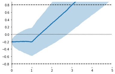
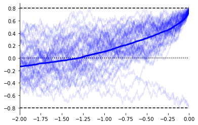
ax = evidently.viz.setup_ddm_plot(model) # Uses model info to draw bounds.
evidently.viz.plot_trace_mean(model, X, ax=ax); # Plots simulations
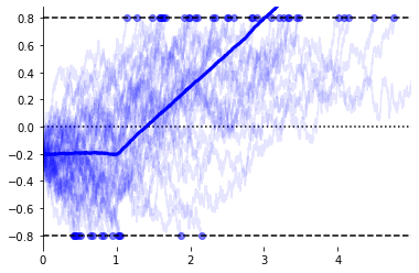
ax = evidently.viz.setup_ddm_plot(model)
evidently.viz.plot_traces(model, X, responses, rts, ax=ax,
                          terminate=True, show_mean=True); # Show raw data
/home/eoin/miniconda3/lib/python3.7/site-packages/evidently/viz.py:162: RuntimeWarning: invalid value encountered in greater
  X.iloc[i, t > rt] = np.nan
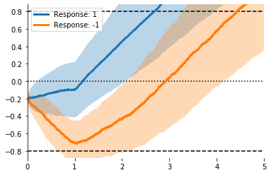
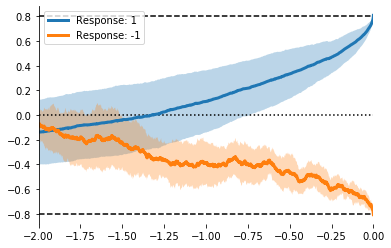
ax = evidently.viz.setup_ddm_plot(model)
for resp in [1, -1]:
    mask = (responses == resp) # Split by response
    evidently.viz.plot_trace_mean(model, X[mask], ax=ax, label='Response: %i' % resp)
plt.legend();
mX = evidently.utils.lock_to_movement(X, rts, duration=2) # Time-lock to threshold crossing
ax = evidently.viz.setup_ddm_plot(model, time_range=(-2, 0))
evidently.viz.plot_traces(model, mX, responses, rts, ax=ax, show_mean=True);
ax = evidently.viz.setup_ddm_plot(model, time_range=(-2, 0))
for resp in [1, -1]:
    mask = responses == resp
    resp_mX = evidently.utils.lock_to_movement(X[mask], rts[mask])
    evidently.viz.plot_trace_mean(model, resp_mX, ax=ax, label='Response: %i' % resp)
plt.legend();
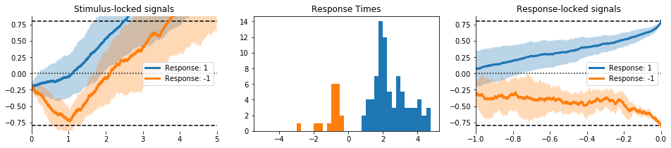
There high-level functions can create multi-axis figures.
evidently.viz.visualise_model(model, model_type='ddm', measure='means');
Interactive Visualisation #
Using the ipywidgets package, we can wrap high level visualisation functions like accum.viz.visualise_ddm in a call to ipywidgets to make them interactive.
To try the interactive plots, download this repository to your own computer, or run the code in the cloud by visiting this Binder notebook.
![]()
from ipywidgets import interact, FloatSlider
def fs(v, low, high, step, desc=''):
    return FloatSlider(value=v, min=low, max=high, step=step, description=desc, continuous_update=False)

def ddm_simulation_plot(t0=1., v=.5, z=0., a=.5, c=.1):
    model = evidently.Diffusion(pars=[t0, v, z, a, c])
    evidently.viz.visualise_model(model)
    title = 't0 = %.1f, Drift = %.1f, Bias = %.1f, Threshold = %.1f; Noise SD = %.1f' % (t0, v, z, a, c)
    plt.suptitle(title, y=1.01)

interact(ddm_simulation_plot,
         t0  = fs(1., 0, 2., .1,   't0'),
         v   = fs(.5, 0, 2., .1,   'Drift'),
         z   = fs(0., -1., 1., .1,  'Bias'),
         a     = fs(.5, 0., 2., .1,   'Threshold'),
         c   = fs(.1, 0., 1., .1,   'Noise SD'));

Here’s the interactive output in GIF form:
Other Models #
The following model classes are currently available:
- Diffusion
- Wald
- HDiffision (Hierarchical Diffusion)
- HWald (Hierarchical Wald)
- Race
See the API for more details.
Road Map #
More Models! #
I have already implemented several of these models, but have to integrate them with the rest of the package.
- Leaky Competing Accumulator model.
- LCA/Race models with > 2 options.
- Leaky/unstable Diffusion.
- Time-varying parameters, including
- Collapsing decision bounds
- Time-varying evidence
- Hierarchical models with regressors that differ across trials.
Reparameterisation #
Ideally, parameterisation with other packages used for fitting accumulator models such as HDDM and PyDDM, (for Python) and rtdists and DMC (for R). This would make it possible to efficiently fit models using those packages, then explore their dynamics here.
Model probably should also specify default parameters.
Visualisation #
There’s no shortage of ways to visualise accumulator models. Future versions will include both more low-level plotting functions and high-level wrappers.
I’ll also be implementing vector field plots, e.g. Figure 2 of Bogacz et al. (2007).
Likelihood #
The evidently.likelihood model contains functions for estimating
the likelihood of data (x) under parameters (\theta) and model (M),
based on the “likelihood-free” technique introduced by
Turner and Sederberg (2007).
These functions aren’t properly tested yet,
and haven’t been documented.