The Monte Carlo Approach

In Monte Carlo approaches, we use random simulations to answer questions that might otherwise require some difficult equations. Confusingly, they’re also known in some fields as numerical approaches, and are contrasted with analytic approaches, where you just work out the correct equation. Wikipedia tells us that, yes, Monte Carlo methods are named after the casino.

The best-known Monte Carlo method is Markov Chain Monte Carlo, which comes up a lot in Bayesian statistics. In this post, I cover a much simpler example. Here’s a simple Monte Carlo example. Let’s say you want to know the area of a circle with a radius of (r). We’ll use a unit circle, (r=1), in this example.

import numpy as np
import matplotlib.pyplot as plt
from matplotlib import rcParams
import seaborn as sns
sns.set_style('whitegrid')
rcParams['figure.figsize'] = (6, 4)
rcParams['font.size'] = 18

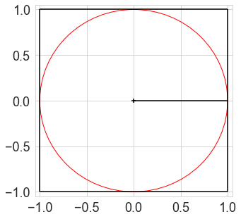
def circle_plot():
    fig, ax = plt.subplots(figsize=(5, 5))
    plt.hlines([-1, 1], -1, 1)
    plt.vlines([-1, 1], -1, 1)
    plt.plot([0, 1], [0, 0], color='k')
    plt.scatter(0, 0, marker='+', color='k')
    plt.xlim(-1.05, 1.05)
    plt.ylim(-1.05, 1.05)
    circle = plt.Circle((0, 0), 1, facecolor='None', edgecolor='r')
    ax.add_artist(circle)
    return fig, ax

circle_plot();

Analytically, you know that the answer is

$$\text{Area} = \pi r^2$$

What if we didn’t know this equation? The Monte Carlo solution is as follows. We know that the area of the bounding square is (2r \times 2r = 4r^2) We need to figure out what proportion of this square is taken up by the circle. To find out, we randomly select a large number of points in the square, and check if they’re within (r) of the center point ([0, 0]).

n = 1000 # Number of points to simulate
x = np.random.uniform(low=-1, high=1, size=n)
y = np.random.uniform(low=-1, high=1, size=n)
# Distance from center (Pythagoras)
dist_from_origin = np.sqrt(x**2 + y**2)
# Check is distance is less than radius
is_in_circle = dist_from_origin < 1

# Plot results
circle_plot()
plt.scatter(x[is_in_circle], y[is_in_circle], color='b', s=2)     # Points in circle
plt.scatter(x[~is_in_circle], y[~is_in_circle], color='k', s=2);  # Points outside circle

m = is_in_circle.mean()
print('%.4f of points are in the circle' % m)

0.7930 of points are in the circle

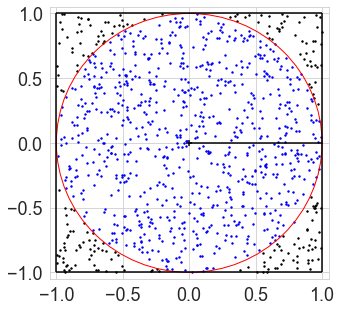
Since the area of the square is (4r^2), and the circle takes up ~(0.78) of the square, the area of the circle is roughly

$$ \begin{align} \text{Area} &\approx 0.78 \times 4r^2 \newline &= 3.14r^2 \newline &\approx \pi r^2 \end{align} $$

We’ve discovered (\pi).