If you take a one-in-n chance \(n\) times (e.g. taking 10 one-in-10 chances), what’s the probability that at least one of them will come off? Somewhat satisfyingly, the answer, regardless of what \(n\) is, turns out to be “around 63%”. Here’s why.

First, some equations.

If you take a one-in-n chance, the probability of it coming off is \( \frac{1}{n} \). For example, if you roll a six-side die, the probability of rolling a 6 is \(\frac{1}{6}\).
The probability of the event not occurring is one minus the probability that it does occur,
\(1 - \frac{1}{n}\).
The probability of trying twice and it not happening is the probability of it not happening the first time, times the probability of it not happening the second time:
\((1 - \frac{1}{n}) \times (1 - \frac{1}{n})\), or \((1 - \frac{1}{n})^2\).
Similarly, the probability of it not happening in \(n\) attempts is
\((1 - \frac{1}{n})^n\)
So the probability that it does happen at least once is the probability that it doesn’t not happen,
\(1 - (1 - \frac{1}{n})^n\)

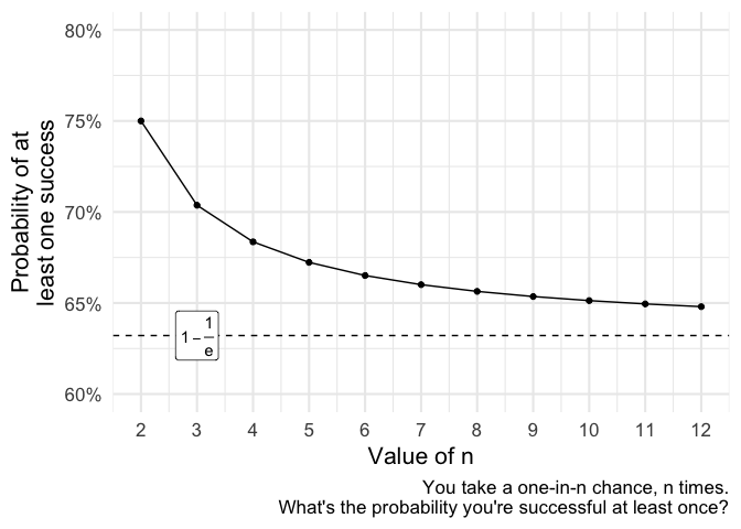
For a one-in-two chance, this works out as
\(1 - (1 - \frac{1}{2})^2 = 1 - \frac{1}{4} = 75\%\).

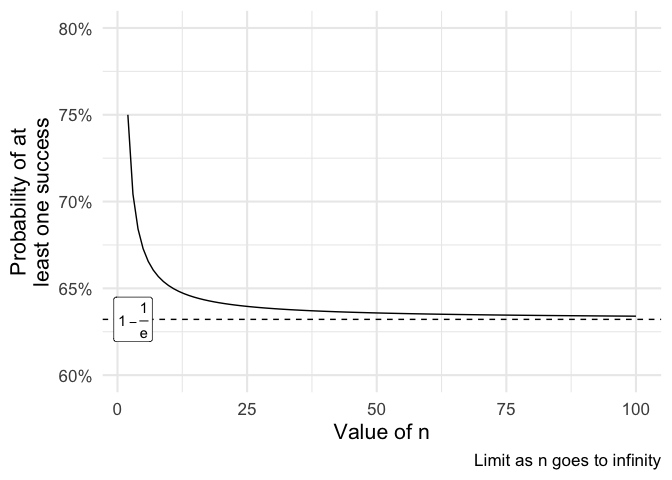
For one-in-three, it’s around \(70.4\%\). For one-in-four, \(68.4\%\). As \(n\) increases, the answer gets closer and closer to \(1 - \frac{1}{e} \approx 63.2\%\), where \(e\) is Euler’s number.

Why \(1 - \frac{1}{e}\)? To be honest, you would have to ask someone better at maths than me, but I think it’s a pretty cool result.

Obligatory XKCD #

xkcd.com/882: “Significant”

Code #

library(tidyverse)
theme_set(theme_minimal(base_size = 16))
ns = 2:12 # Values of n

# Probability of one or more successes
prob_of_success = function(n){
  1 - (1 - 1/n)^n
}
probs = prob_of_success(ns)
limit_val = 1 - (1 / exp(1))

df = data.frame(
  n = ns,
  prob = probs
)

ggplot(df, aes(n, prob)) +
  geom_path() +
  geom_point() +
  coord_cartesian(ylim=c(.6, .8)) +
  scale_x_continuous(breaks=ns) +
  scale_y_continuous(labels=scales::percent) +
  geom_hline(yintercept=limit_val, linetype='dashed') +
  annotate('label', x=3, y=limit_val, label=expression(1  -  frac(1,'e'))) +
  labs(x = "Value of n", y="Probability of at\nleast one success",
       caption = "You take a one-in-n chance, n times.\nWhat's the probability you're successful at least once?")

ggplot(data.frame(n=2:100), aes(x=n)) +
  geom_function(fun=prob_of_success) +
  coord_cartesian(ylim=c(.6, .8)) +
  # scale_x_continuous(breaks=ns) +
  scale_y_continuous(labels=scales::percent) +
  geom_hline(yintercept=limit_val, linetype='dashed') +
  annotate('label', x=3, y=limit_val, label=expression(1  -  frac(1,'e'))) +
  labs(x = "Value of n", y="Probability of at\nleast one success",
       caption = "Limit as n goes to infinity")

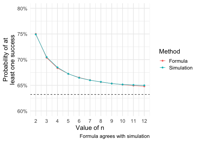
Don’t trust my formula? I don’t blame you, I never trust anything I figure out myself. That’s why I double check it against a simulation.

sim_func = function(n, nsims=100000){
  outcomes = rbinom(n=nsims, size=n, prob=1/n)
  mean(outcomes > 0)
}
df$sim_p = map_dbl(ns, sim_func)

df %>%
  pivot_longer(-n) %>%
  mutate(name = ifelse(name=='prob', 'Formula', 'Simulation')) %>%
  ggplot(aes(n, value, color=name)) +
  geom_path() + 
  geom_point() +
  coord_cartesian(ylim=c(.6, .8)) +
  scale_x_continuous(breaks=ns) +
  scale_y_continuous(labels=scales::percent) +
  geom_hline(yintercept=limit_val, linetype='dashed') +
  labs(x = "Value of n", y="Probability of at\nleast one success", color = "Method",
       caption = "Formula agrees with simulation")